
A language model normally accepts discrete tokens. Hand it a photograph and the pixels do not automatically become “a snowy mountain reflected in a lake,” much less “compare what the two people on the left are doing.” The obvious solution seems to be training one enormous model to learn vision and language from scratch. LLaVA took a cheaper and more revealing route: retain a vision encoder that already knows how to represent images, retain a language model that already knows how to converse, and train a small bridge between them.
That bridge was a single linear projection in the first LLaVA and a two-layer MLP in LLaVA-1.5. Its importance does not come from a small matrix creating visual intelligence out of nowhere. It changes the interface contract between two pretrained systems: convert the vision encoder’s grid features into vectors that can occupy positions in the language model’s context, then use visual-instruction data to teach the language model what to do with those vectors.
CLIP Built Language Coordinates for Images, Not a Conversation System
LLaVA’s visual side starts with CLIP. CLIP trains an image encoder and a text encoder on paired images and text. The objective pulls matching pairs together and pushes mismatched pairs apart. OpenAI trained it on 400 million web image-text pairs and framed the proxy task as identifying the correct caption among the text candidates in a batch.
This creates an open semantic coordinate system. A conventional classifier chooses from a predetermined label set. CLIP can instead compare an image with descriptions such as “a snowy mountain reflected in a lake” or “a handwritten menu,” so its visual representation is not confined to one fixed taxonomy.
But matching an image to a sentence is not the same as holding a multi-turn conversation about the image. CLIP’s core output is similarity. It does not generate long answers or follow instructions such as “count only the red objects” and “explain first, then answer.” LLaVA does not ask CLIP to answer questions. It borrows CLIP’s visual features and delegates generation and instruction following to a language model that already has those capabilities.
The Image Is Not Translated Into Words
In a common LLaVA-1.5 configuration, an image enters CLIP ViT-L/14 at 336 pixels. The ViT divides the 336×336 image into 14×14 patches, producing a (24\times24=576) grid. The vision encoder emits one feature vector per grid position. A connector (P) then projects the visual dimension into the language model’s word-embedding dimension:
\[ H_v=P(Z_v), \qquad Z_v=g(X_v). \]The vectors in (H_v) are often called visual tokens, but they are not vocabulary tokens and do not each name a readable word. They are continuous vectors with the same width as the model’s text embeddings. The system places them beside the question embeddings, allowing the autoregressive language model to attend to image regions and the textual prompt in one sequence.
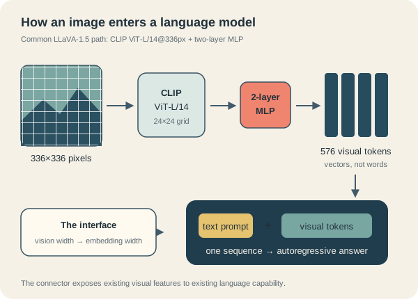
Figure 1: LLaVA projects CLIP grid features into continuous visual tokens that can enter the language model context
This design avoids a separate multimodal decoder and does not add a new cross-attention block to every language-model layer. The tradeoff is that visual information consumes token budget inside the LLM. A finer image grid may preserve more detail, but it also lengthens the sequence and increases prefill attention and KV-cache work. A small connector does not make the whole multimodal inference path cheap.
Two Training Stages Teach Two Different Contracts
The original LLaVA uses two stages. Stage one takes 595K image-text pairs filtered from CC3M and turns each pair into a simple request such as “briefly describe this image.” Both the vision encoder and the language model stay frozen; only the projection matrix is updated. This stage is not teaching conversation. It finds a visual representation that the frozen language model can consume. The paper describes it as training a compatible visual tokenizer for the LLM.
Stage two switches to 158K visual-instruction examples spanning conversation, detailed description, and complex reasoning. The vision encoder remains frozen, while the connector and language model are updated together. The autoregressive loss is applied to the assistant answer tokens, teaching the model the behavior “image plus instruction produces an appropriate response.”
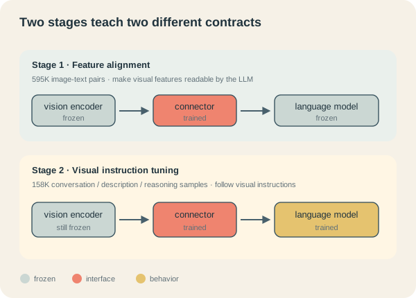
Figure 2: Stage one aligns the interface; stage two trains the connector and language model to follow visual instructions
It is misleading to collapse these stages into “train on image-text data.” The first solves representation compatibility: how should a feature for the mountain region enter the LLM’s vector space? The second solves an interaction contract: how should the answer change when the same image is paired with “describe the scene,” “count the people,” or “explain what is unusual”? One gets the signal through the door; the other teaches the model to use it according to human intent.
A Small Bridge Works Because Both Banks Already Do Most of the Work
The connector’s size does not mean vision and language are naturally aligned. Most expensive capabilities already exist. CLIP has learned associations between many visual concepts and language semantics. Vicuna inherits a language model’s knowledge, generation, and instruction-following behavior. The projection does not need to relearn object recognition or grammar. It needs to find an interface between two useful representation spaces, with later tuning adapting the LLM to that interface.
LLaVA-1.5 provides a valuable engineering result. Replacing the original linear projection with a two-layer MLP, raising CLIP input resolution to 336 pixels, and adding public academic VQA data with concise response-format prompts produced a strong open baseline across 11 benchmarks. The paper reports that its final 13B checkpoint used about 1.2 million public samples and completed full training in roughly one day on a single eight-A100 node.
That result does not prove that simpler connectors are universally superior. It supports a narrower claim: when the vision encoder, language model, and data are already strong, connector complexity may not be the first bottleneck. BLIP-2 illustrates another valid design. Its Q-Former uses learned queries and cross-attention to extract a fixed number of language-relevant features from the image encoder. LLaVA preserves the patch grid and favors a simple, rapidly iterable interface; Q-Former actively compresses information, trading more structure for a token count that does not directly grow with the input grid. The right bridge depends on fidelity, compute, and data—not on an abstract ranking of architectural sophistication.
Visual-Instruction Data Changed the Way the Model Could Be Used
The source of LLaVA’s 158K instruction examples is unusually instructive. The GPT-4 version available to the researchers accepted only text, so they did not show the teacher raw images. They represented each image through captions and bounding boxes, then asked GPT-4 to generate conversations, detailed descriptions, and complex reasoning questions around that symbolic description. The student still saw the real image during training.
This pipeline reframed existing image-text data. The old question was “what caption belongs to this image?” The new question was “what might a user ask the assistant to do with this image?” That behavioral change mattered more than the raw sample count. In the paper’s ablation on LLaVA-Bench (COCO), the system without visual instruction tuning received an overall score of 21.5; the full instruction dataset raised it to 85.1. These are scores from a specific setup using text-only GPT-4 as judge and reference, not percentages of universal capability. Within that setup, however, the gap clearly shows that describing images and following instructions about images are different skills.
Synthetic instruction data also has a hard boundary. The teacher saw captions and boxes rather than pixels. If the symbolic description omitted a fine detail, the generated question and answer could not reliably recover that visual evidence. The student may learn the teacher’s verbal preferences and reasoning templates without improving fine perception. Synthetic instructions broaden behavioral coverage; they do not replace grounded OCR data, detailed region annotations, or verified spatial relations.
Visual Tokens Are Both an Information Budget and a Compute Bill
Sending every patch into the LLM is direct and preserves local representations. But patch count grows quadratically with image side length. With patch size 14, a square 224-pixel image produces 256 grid positions, 336 pixels produces 576, and 672 pixels produces 2,304. Doubling each side quadruples the visual tokens.
If the prompt has (N_t) text tokens and the image contributes (N_v) visual tokens, a standard self-attention layer sees length (N_t+N_v). Its attention matrix scales roughly with ((N_t+N_v)^2), while KV cache scales with the total token count. Real systems can alter the bill with tiling, downsampling, token merging, sparse attention, or a visual resampler, but none eliminates the conflict between information density and computation.
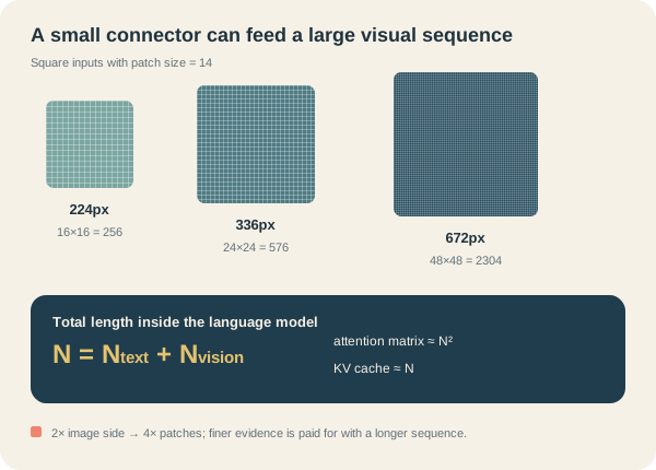
Figure 3: Connector parameters can stay small while visual-token length and attention cost grow rapidly with resolution
This is why “higher resolution” is not enough to compare multimodal systems. We also need to ask how many tokens an image creates, how multiple images accumulate, whether visual tokens consume text context, whether they are compressed before entering the LLM, and whether a latency number measures image encoding, prefill, or autoregressive decoding. A maximum supported resolution is an input limit, not a recommendation to use that resolution for every request.
Fluent Language Makes Visual Errors Harder to Notice
Vision-language models combine uncertain perception with confident language generation. The original LLaVA paper describes a telling failure: a refrigerator contains strawberries and yogurt, but no strawberry-flavored yogurt; the model still answers yes when asked whether that flavor is present. It composes two co-occurring concepts into a relationship that the image does not contain. The authors describe the system as sometimes seeing a “bag of patches” without capturing the complex semantics.
The error can enter at three points. The vision encoder may fail to preserve small text, counts, or exact locations. The connector may not map the relevant detail into directions the LLM can use. The language model may fill missing evidence with a plausible textual prior. The final fluent sentence does not reveal which layer failed.
Practical evaluation should therefore separate perception, localization, OCR, relations, and generation. High-stakes systems may need traceable regions, external detectors, or abstention rather than a single score for how human-like the answer sounds. LLaVA itself notes inherited bias from its vision and language backbones, image-grounding hallucination, and the difficulty of evaluating a system that spans two modalities.
LLaVA’s most durable contribution may not be a checkpoint that still tops today’s leaderboards. It is a minimal, reproducible blueprint: a strong vision encoder sees, a strong language model speaks, a lightweight interface puts their representations in one sequence, and instruction data defines the new interaction. The work showed how quickly multimodal capability could emerge by composing foundation models. It also showed why the bridge’s parameter count tells us little about the information, training protocol, compute, and failure attribution carried across it.
References
- Radford et al., Learning Transferable Visual Models From Natural Language Supervision, ICML 2021.
- OpenAI, CLIP: Connecting Text and Images.
- Liu et al., Visual Instruction Tuning, NeurIPS 2023 Oral.
- Liu et al., Improved Baselines with Visual Instruction Tuning, 2023.
- LLaVA authors, Official LLaVA Code and Training Instructions.
- Li et al., BLIP-2: Bootstrapping Language-Image Pre-training with Frozen Image Encoders and Large Language Models, ICML 2023.